n-step Bootstrapping

이 포스트에서는 TD method의 확장된 형태인 $n$-step TD methods를 간략히 소개한다.

What is $n$-step TD method

$n$-step TD method는 1-step TD method와 Monte Carlo (MC) method를 통합한 방법이다. $n$-step TD method는 일종의 스펙트럼으로 양 끝단에 각각 1-step TD와 MC method가 존재한다. 실제 1-step TD나 MC method가 항상 좋은 performance를 내는건 아니다. 따라서 보다 일반적인 n-step TD method에 대해 알아둘 필요가 있다.

이전 포스트에서 TD method는 MC method와 Dynamic Programming (DP)의 아이디어를 결합한 방법이라고 소개했었다. $n$-step method 역시 동일하다. 즉, sampling과 bootstrapping을 통해 training이 이루어진다. 다만 1-step TD와의 차이점은 bootstrapping이 이루어지는 time step이 1개가 아니라 여러 개일 뿐이다.

$n$-step TD Prediction

MC method는 episode를 완전히 고려하기 때문에 전체 reward를 알고 있어 실제 return을 구할 수 있었다.

\[G_t \doteq R_{t+1} + \gamma R_{t+2} + \gamma^2 R_{t+3} + \cdots + \gamma^{T-t-1}R_T\]

$T$는 episode의 last time step이다. 그런데 1-step TD method는 episode 전체가 아니라 sampling된 단 하나의 transition 고려하기 때문에 next reward $R_{t+1}$만 구할 수 있다. 따라서 아직 sampling 되지 않은 time step들의 discounted reward들을 아래와 같이 next state에서의 추정치로 근사해 처리한다.

\[G_{t:t+1} \doteq R_{t+1} + \gamma V_t(S_{t+1})\]

$G_{t:t+1}$은 time step $t$에서 $t+1$까지의 transition이 발생했을 때의 target으로 1-step return이라고 한다. 참고로 MC method의 target은 실제 return $G_t$이다. 우리는 위 1-step TD method의 target을 $n$-step으로 확장할 것이다. 먼저 아래 backup diagram을 보자.

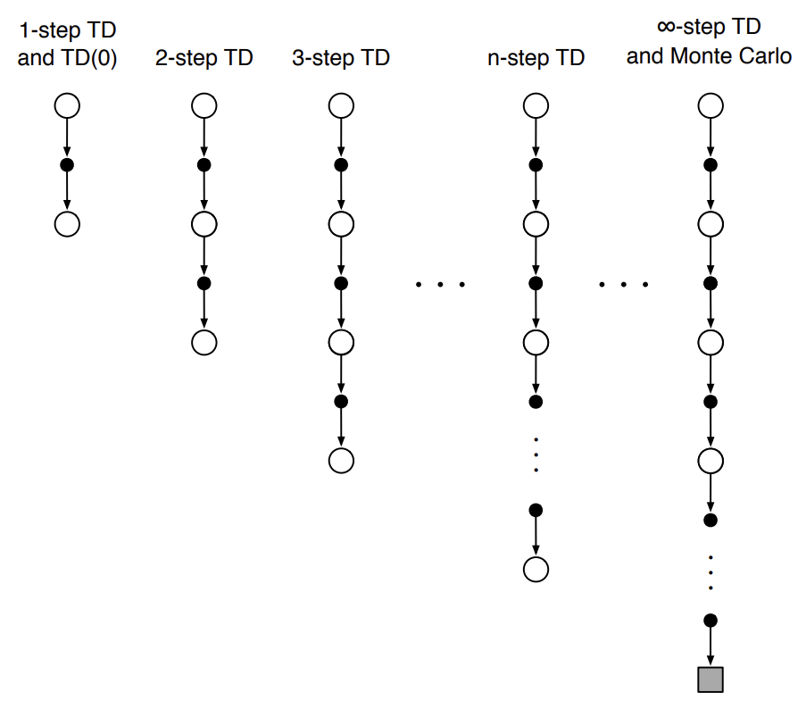Fig 1. Backup diagrams of $n$-step methods.
(Image source: Sec 7.1 Sutton & Barto (2018).)

위 backup diagram을 보면 알 수 있지만 1-step TD 수행 시 실제 reward는 $R_{t+1}$만 획득할 수 있다. 2-step TD 수행 시 $R_{t+1}$과 $R_{t+2}$만 획득할 수 있다. 획득하지 못한 나머지 reward는 기존에 학습된 추정치로 대체한다. 즉, 2-step TD 수행 시 $S_{t+2}$에 위치할 것이기 때문에 $V(S_{t+2})$를 사용한다. 아래는 2-step TD method의 target이다.

\[G_{t:t+2} \doteq R_{t+1} + \gamma R_{t+2} + \gamma^2 V_{t+1}(S_{t+2})\]

이를 $n$-step TD method로 일반화하면 아래와 같다.

\[G_{t:t+n} \doteq R_{t+1} + \gamma R_{t+2} + \cdots + \gamma^{n-1} R_{t+n} + \gamma^n V_{t+n-1}(S_{t+n})\]

위 $n$-step TD method의 target을 $n$-step return이라고 한다. 정리하면 $n$-step return은 실제 return의 근사치로, $n$-step 이후 잘려진 뒤 $V_{t+n-1}(S_{t+n})$에 의해 보정된 값이다. 이 때 $t + n \geq T$일 경우, episode의 termination을 넘어갔기 때문에 보정된 값은 0이 되어 실제 return이 된다.

\[G_{t:t+n} \doteq G_t, \quad \text{if } t + n \geq T\]

$n$-step return은 $n$-step 이후의 $R_{t+n}$과 이전에 계산된 $V_{t+n-1}$이 발견이 되어야만 계산할 수 있다. 따라서 $t+n$ time step 이후에만 $G_{t:t+n}$을 이용할 수 있다. 아래는 $n$-step return을 사용해 state value를 추정하는 prediction update rule이다.

\[V_{t+n}(S_t) \doteq V_{t+n-1}(S_t) + \alpha [G_{t:t+n} - V_{t+n-1}(S_t)]\]

이 때 $s \neq S_t$인 모든 state의 value는 변하지 않는다. 위 update rule이 $n$-step TD이다. episode의 첫 $n-1$ step까지는 어떤 변화도 발생하지 않는다는 사실을 꼭 기억하길 바란다.

$\text{Algorithm: $n$-step TD for estimating } V \approx v_\pi$

\(\begin{align*} & \textstyle \text{Input: a policy } \pi \\ & \textstyle \text{Algorithm parameters: step size } \alpha \in (0, 1] \text{, a positive integer } n \\ & \textstyle \text{Initialize } V(s) \text{ arbitrarily, for all } s \in \mathcal{S} \\ & \textstyle \text{All store and access operations (for } S_t \text{ and } R_t \text{) can take their index mod } n+1 \\ \\ & \textstyle \text{Loop for each episode:} \\ & \textstyle \qquad \text{Initialize and store } S_0 \neq \text{terminal} \\ & \textstyle \qquad T \leftarrow \infty \\ & \textstyle \qquad \text{Loop for } t = 0, 1, 2, \dotso : \\ & \textstyle \qquad\qquad \text{If } t < T \text{, then:} \\ & \textstyle \qquad\qquad\qquad \text{Take an action according to } \pi(\cdot \vert S_t) \\ & \textstyle \qquad\qquad\qquad \text{Observe and store the next reward as } R_{t+1} \text{ and the next state as } S_{t+1} \\ & \textstyle \qquad\qquad\qquad \text{If } S_{t+1} \text{ is terminal, then } T \leftarrow t + 1 \\ & \textstyle \qquad\qquad \tau \leftarrow t - n + 1 \qquad \text{($\tau$ is the time whose state's estimate is being updated)} \\ & \textstyle \qquad\qquad \text{If $\tau \geq 0$:} \\ & \textstyle \qquad\qquad\qquad G \leftarrow \sum_{i=\tau + 1}^{\min(\tau + n, T)} \gamma^{i - \tau - 1}R_i \\ & \textstyle \qquad\qquad\qquad \text{If } \tau + n < T \text{, then: } G \leftarrow G + \gamma^n V(S_{\tau + n}) \qquad (G_{\tau : \tau + n}) \\ & \textstyle \qquad\qquad\qquad V(S_\tau) \leftarrow V(S_\tau) + \alpha [G - V(S_\tau)] \\ & \textstyle \qquad \text{until } \tau = T - 1 \end{align*}\)

위 알고리즘을 보면 $n$-step transition이 발생할 때는 $t = n-1$일 때로 이 때 부터 value function의 update가 수행된다.

$n$-step Sarsa

이제 $n$-step method의 control에 대해 알아보자. 가장 먼저 알아볼 것은 n-step Sarsa이다. Sarsa는 on-policy method이며 여기서는 단지 1-step이 아닌 $n$-step으로 확장했을 뿐이다.

핵심 아이디어는 MC나 1-step TD method와 동일하게 state value 추정을 action value 추정으로 전환하는 것이다. 이에 따라 모든 시작과 끝은 state가 아니라 action이 된다. 아래는 $n$-step Sarsa에 대한 backup diagram이다.

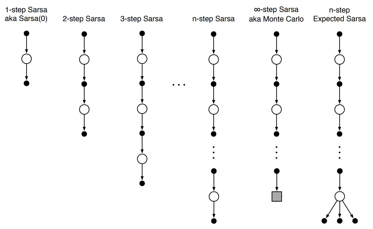Fig 2. Backup diagrams of $n$-step Sarsa.
(Image source: Sec 7.2 Sutton & Barto (2018).)

이제 $n$-step Sarsa에서 사용하기 위한 $n$-step return을 action value에 관해 정의해보자. 단지, $n$-step TD Prediction의 $n$-step return에서 $V$를 $Q$로 바꿔주기만 하면 된다.

\[G_{t:t+n} \doteq R_{t+1} + \gamma R_{t+2} + \cdots + \gamma^{n-1} R_{t+n} + \gamma^n Q_{t+n-1}(S_{t+n}, A_{t+n}), \quad n \geq 1, 0 \leq t < T - n\]

단, $t + n \geq T$일 때 $G_{t:t+n} \doteq G_t$이다. 위 $n$-step return for Sarsa를 바탕으로 $n$-step Sarsa의 update rule을 정의해보자.

\[Q_{t+n}(S_t,A_t) \doteq Q_{t+n-1}(S_t,A_t) + \alpha [G_{t:t+n} - Q_{t+n-1}(S_t, A_t)], \quad 0 \leq t < T\]

역시 마찬가지로 $s \neq S_t$ or $a \neq A_t$인 모든 $s, a$에 대한 value function은 변하지 않는다.

아래는 1-step Sarsa와 $n$-step Sarsa를 비교하는 그림이다. 파란색 화살표는 목표 G에 도달했을 떄 증가하는 action value를 나타낸다.

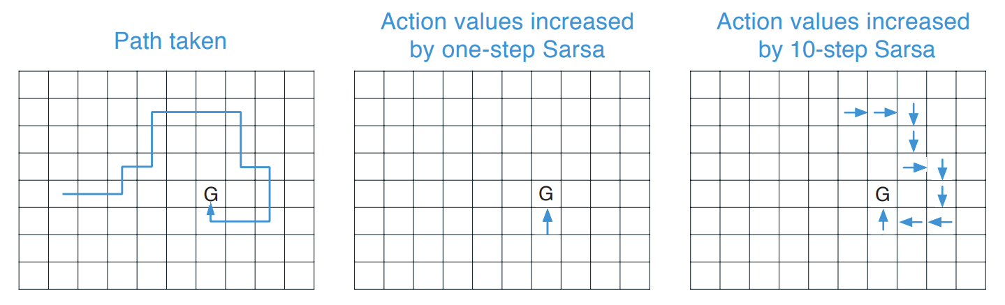Fig 3. Comparison of 1-step and $n$-step Sarsa.
(Image source: Sec 7.2 Sutton & Barto (2018).)

위 그림을 보면 알 수 있지만 목표 G에 도달했을 때 1-step Sarsa는 바로 직전 state에서의 action value만 증가하지만 $n$-step Sarsa는 sequence의 마지막 $n$개의 action만큼 증가한다. 이로 인해 하나의 episode로부터 더 많은 학습이 가능해진다.

아래는 $n$-step Sarsa의 알고리즘이다.

$\text{Algorithm: $n$-step Sarsa for estimating } Q \approx q_\ast \text{ or } q_\pi$

\(\begin{align*} & \textstyle \text{Initialize } Q(s,a) \text{ arbitrarily, for all } s \in \mathcal{S}, a \in \mathcal{A} \\ & \textstyle \text{Initialize $\pi$ to be $\epsilon$-greedy with respect to $Q$, or to a fixed given policy} \\ & \textstyle \text{Algorithm parameters: step size } \alpha \in (0, 1] \text{, small $\epsilon > 0$, a positive integer $n$} \\ & \textstyle \text{All store and access operations (for $S_t$, $A_t$, and $R_t$) can take their index mod $n+1$} \\ \\ & \textstyle \text{Loop for each episode}: \\ & \textstyle \qquad \text{Initialize and store } S_0 \neq \text{terminal} \\ & \textstyle \qquad \text{Select and store an action } A_0 \sim \pi(\cdot \vert S_0) \\ & \textstyle \qquad T \leftarrow \infty \\ & \textstyle \qquad \text{Loop for } t = 0, 1, 2, \dotso \text{:} \\ & \textstyle \qquad\vert\qquad \text{If $t < T$, then:} \\ & \textstyle \qquad\vert\qquad\qquad \text{Take action } A_t \\ & \textstyle \qquad\vert\qquad\qquad \text{Observe and store the next reward as $R_{t+1}$ and the next state as $S_{t+1}$} \\ & \textstyle \qquad\vert\qquad\qquad \text{If $S_{t+1}$ is terminal, then:} \\ & \textstyle \qquad\vert\qquad\qquad\qquad T \leftarrow t + 1 \\ & \textstyle \qquad\vert\qquad\qquad \text{else:} \\ & \textstyle \qquad\vert\qquad\qquad\qquad \text{Select and store an action } A_{t+1} \sim \pi(\cdot \vert S_{t+1}) \\ & \textstyle \qquad\vert\qquad \tau \leftarrow t - n + 1 \qquad (\tau \text{ is the time whose estimate is being updated}) \\ & \textstyle \qquad\vert\qquad \text{If $\tau \geq 0$:} \\ & \textstyle \qquad\vert\qquad\qquad G \leftarrow \sum_{i = \tau + 1}^{\min(\tau + n, T)} \gamma^{i - \tau - 1}R_i \\ & \textstyle \qquad\vert\qquad\qquad \text{If } \tau + n < T \text{, then } G \leftarrow G + \gamma^n Q(S_{\tau + n}, A_{\tau + n}) \qquad (G_{\tau : \tau + n}) \\ & \textstyle \qquad\vert\qquad\qquad Q(S_\tau, A_\tau) \leftarrow Q(S_\tau, A_\tau) + \alpha [G - Q(S_\tau, A_\tau)] \\ & \textstyle \qquad\vert\qquad\qquad \text{If $\pi$ is being learned, then ensure that $\pi(\cdot \vert S_\tau)$ is $\epsilon$-greedy wrt $Q$} \\ & \textstyle \qquad \text{until } \tau = T - 1 \\ \end{align*}\)

$n$-step Expected Sarsa

$n$-step Expected Sarsa 역시 어렵지 않게 구할 수 있다.. Fig.2를 보면 알 수 있지만 Sarsa와 동일하게 진행되나 마지막 $n$-step에서 모든 action value에 대한 expected value를 고려한다. 아래는 임의의 state $s$에서 action value 추정치를 통해 획득할 수 있는 expected approximate value이다.

\[\bar{V}_t(s) \doteq \sum_a \pi(a \vert s)Q_t(s,a), \quad \text{for all } s \in \mathcal{S}\]

이 때 $\pi$는 target policy이다. 위 수식을 바탕으로 Expected Sarsa에 대한 $n$-step return을 구할 수 있다.

\[G_{t:t+n} \doteq R_{t+1} + \cdots + \gamma^{n-1}R_{t+n} + \gamma^n \bar{V}_{t+n-1}(S_{t+n}), \quad t + n < T\]

위 수식을 바탕으로 $n$-step Sarsa 알고리즘을 약간만 변형하면 $n$-step Expected Sarsa 알고리즘을 쉽게 구할 수 있다.

$n$-step Off-policy Learning

off-policy learning은 behavior policy $b$에 따라 sampling 한 뒤, target policy $\pi$에 대한 value function을 학습 하는 방법이다. off-policy method에서 behavior policy와 target policy의 distribution이 다르기 때문에 importance-sampling 기법을 사용했었다. importance-sampling ratio는 어떤 trajectory의 action들을 두 policy에 따라 선택할 상대적 확률이다.¹

\[\rho_{t:h} \doteq \prod_{k=t}^{\min(h, T-1)} \dfrac{\pi(A_k \vert S_k)}{b(A_k \vert S_k)}\]

아래는 $S_t$가 주어져있을 때 $n$-step transition으로 생성된 trajectory이다.

\[A_t, S_{t+1}, A_{t+1}, \dots, A_{t+n-1}, S_{t+n}\]

이 때 off-policy에서는 아래와 같이 importance-sampling ratio $\rho_{t:t+n-1}$을 통해 $n$-step TD error에 가중치를 부여하여 update를 수행할 수 있다.

\[V_{t+n}(S_t) \doteq V_{t+n-1}(S_t) + \alpha \rho_{t:t+n-1}[G_{t:t+n} - V_{t+n-1}(S_t)], \quad 0 \leq t < T\]

이를 바탕으로 off-policy $n$-step Sarsa를 정의할 수 있다. 마찬가지로 state value를 action value로 전환하면 된다. 다만 importance-sampling ratio을 고려할 때 주의할 점이 있다. state value 추정과 action value 추정 시의 trajectory가 달라 importance-sampling ratio가 다르다. action value를 추정할 때는 state action pair $S_t, A_t$가 주어져 있으며, Sarsa이기 때문에 trajectory의 마지막 state에서도 action을 선택한다. 아래는 Sarsa의 $n$-step transition trajectory이다.

\[S_{t+1}, A_{t+1}, \dots, A_{t+n-1}, S_{t+n}, A_{t+n}\]

따라서 우리가 고려해야할 importance-sampling ratio는 $\rho_{t+1:t+n}$이다. 아래는 off-policy Sarsa의 update rule이다.

\[Q_{t+n}(S_t, A_t) \doteq Q_{t+n-1}(S_t, A_t) + \alpha \rho_{t+1:t+n}[G_{t:t+n} - Q_{t+n-1}(S_t, A_t)], \quad 0 \leq t < T\]

importance-sampling ratio는 subsequent action에 대해서만 고려한다는 사실을 꼭 기억하길 바란다. 아래는 off-policy $n$-step Sarsa 알고리즘이다.

$\text{Algorithm: Off-policy $n$-step Sarsa for estimating } Q \approx q_\ast \text{ or } q_\pi$

\(\begin{align*} & \textstyle \text{Input: an arbitrary behavior policy $b$ such that $b(a \vert s) > 0$, for all } s \in \mathcal{S}, a \in \mathcal{A} \\ & \textstyle \text{Initialize } Q(s,a) \text{ arbitrarily, for all } s \in \mathcal{S}, a \in \mathcal{A} \\ & \textstyle \text{Initialize $\pi$ to be greedy with respect to $Q$, or as a fixed given policy} \\ & \textstyle \text{Algorithm parameters: step size } \alpha \in (0, 1] \text{, a positive integer $n$} \\ & \textstyle \text{All store and access operations (for $S_t$, $A_t$, and $R_t$) can take their index mod $n+1$} \\ \\ & \textstyle \text{Loop for each episode}: \\ & \textstyle \qquad \text{Initialize and store } S_0 \neq \text{terminal} \\ & \textstyle \qquad \text{Select and store an action } A_0 \sim b(\cdot \vert S_0) \\ & \textstyle \qquad T \leftarrow \infty \\ & \textstyle \qquad \text{Loop for } t = 0, 1, 2, \dotso \text{:} \\ & \textstyle \qquad\vert\qquad \text{If $t < T$, then:} \\ & \textstyle \qquad\vert\qquad\qquad \text{Take action } A_t \\ & \textstyle \qquad\vert\qquad\qquad \text{Observe and store the next reward as $R_{t+1}$ and the next state as $S_{t+1}$} \\ & \textstyle \qquad\vert\qquad\qquad \text{If $S_{t+1}$ is terminal, then:} \\ & \textstyle \qquad\vert\qquad\qquad\qquad T \leftarrow t + 1 \\ & \textstyle \qquad\vert\qquad\qquad \text{else:} \\ & \textstyle \qquad\vert\qquad\qquad\qquad \text{Select and store an action } A_{t+1} \sim b(\cdot \vert S_{t+1}) \\ & \textstyle \qquad\vert\qquad \tau \leftarrow t - n + 1 \qquad (\tau \text{ is the time whose estimate is being updated}) \\ & \textstyle \qquad\vert\qquad \text{If $\tau \geq 0$:} \\ & \textstyle \qquad\vert\qquad\qquad \rho \leftarrow \prod_{i = \tau + 1}^{\min(\tau + n, T-1)} \frac{\pi(A_i \vert S_i)}{b(A_i \vert S_i)} \qquad (\rho_{\tau + 1:\tau + n}) \\ & \textstyle \qquad\vert\qquad\qquad G \leftarrow \sum_{i = \tau + 1}^{\min(\tau + n, T)} \gamma^{i - \tau - 1}R_i \\ & \textstyle \qquad\vert\qquad\qquad \text{If } \tau + n < T \text{, then: } G \leftarrow G + \gamma^n Q(S_{\tau + n}, A_{\tau + n}) \qquad (G_{\tau : \tau + n}) \\ & \textstyle \qquad\vert\qquad\qquad Q(S_\tau, A_\tau) \leftarrow Q(S_\tau, A_\tau) + \alpha \rho [G - Q(S_\tau, A_\tau)] \\ & \textstyle \qquad\vert\qquad\qquad \text{If $\pi$ is being learned, then ensure that $\pi(\cdot \vert S_\tau)$ is greedy wrt $Q$} \\ & \textstyle \qquad \text{until } \tau = T - 1 \\ \end{align*}\)

참고로 위 알고리즘은 Reinforcement: An Introduction (2020)에 소개된 알고리즘이다. 2018에 있는 알고리즘과 살짝 다른데 2020 버전이 올바른 알고리즘으로 보인다.

off-policy Expected Sarsa의 경우 위 알고리즘에서 importance-sampling ratio $\rho_{t+1:t+n}$ 대신에 $\rho_{t+1:t+n-1}$을 사용하고 $n$-step return Expected Sarsa version을 사용하면 된다. importance-sampling ratio에서 마지막 action을 고려하지 않는 이유는 아래와 같다.

This is because in Expected Sarsa all possible actions are taken into account in the last state; the one actually taken has no e↵ect and does not have to be corrected for.²

$n$-step Tree Backup

importance sampling은 off-policy learning을 가능하게 하지만 분산이 커질 수 있다는 단점이 있다. importance sampling을 사용하지 않고 off-policy learning을 가능하게 해주는 방법이 있는데 바로 tree-backup algorithm이다. 아래는 3개의 sample transition과 2개의 sample action을 나타낸 backup diagram이다. 각 state node의 사이드에 달려 있는 action node들은 sampling 시에 선택되지 않은 action을 나타낸다.

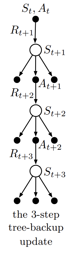Fig 4. 3-step tree-backup diagram.
(Image source: Sec 7.5 Sutton & Barto (2018).)

지금까지 diagram에서 top node의 action value를 추정할 때 아래 node를 쭉 따라 획득한 discounted reward들과 가장 아래 node의 value를 결합한 값을 사용했었다. tree-backup algorithm은 이러한 것들에 추가적으로 위 backup diagram에서 각 state들의 사이드에 달려 있는 action node에 해당하는 value 추정치 또한 고려한다.

좀 더 구체적으로 보자. 먼저, 각 sample transition에서 선택되지 않은 action $a \neq A_{t+1}$들은 target policy $\pi$에 의해 추정된 action value에 가중치 $\pi(a \vert S_{t+1})$을 부여한다. 실제로 선택된 action $A_{t+1}$은 다음 단계의 모든 action에 $\pi(A_{t+1} \vert S_{t+1})$을 가중치로 부여한다. 이는 재귀적으로 수행된다.

이제 구체적인 $n$-step tree-backup algorithm에 대한 수식을 보자. 먼저 1-step return은 아래와 같이 정의된다. 이 때 1-step return은 Expected Sarsa의 return과 동일하다.

\[G_{t:t+1} \doteq R_{t+1} + \gamma \sum_a \pi(a \vert S_{t+1})Q_t(S_{t+1}, a), \quad t < T-1\]

2-step tree-backup return은 아래와 같이 정의된다.

\[\begin{align*} G_{t:t+2} &\doteq R_{t+1} + \gamma \sum_{a \neq A_{t+1}} \pi(a \vert S_{t+1})Q_{t+1}(S_{t+1}, a) \\ &+ \gamma \pi (A_{t+1} \vert S_{t+1})\Big(R_{t+2} + \gamma \sum_a \pi(a \vert S_{t+2})Q_{t+1}(S_{t+2},a) \Big) \\ &= R_{t+1} + \gamma \sum_{a \neq A_{t+1}} \pi(a \vert S_{t+1})Q_{t+1}(S_{t+1},a) + \gamma \pi(A_{t+1} \vert S_{t+1})G_{t+1:t+2}, \quad t < T - 2 \end{align*}\]

$n$-step tree-backup return (target)은 아래와 같이 정의된다. 단지 위 수식을 $n$-step에 대한 재귀적 형태로 바꿔주면 된다.

\[G_{t:t+n} \doteq R_{t+1} + \gamma \sum_{a \neq A_{t+1}} \pi(a \vert S_{t+1})Q_{t+n-1}(S_{t+1}, a) + \gamma \pi(A_{t+1} \vert S_{t+1})G_{t+1:t+n}, \quad t < T - 1, n \geq 2\]

참고로 위 수식에서 $t < T-1$인 이유는 $G_{t+1:t+n}$에서 sub-sequence가 처리되기 때문이다. $n=1$인 경우는 $G_{t:t+1}$을 사용하면 된다. 또한 $G_{T-1:t+n} \doteq R_T$로 정의된다. 위에서 정의한 target을 일반적인 $n$-step Sarsa update rule에 적용하면 아래와 같다.

\[Q_{t+n}(S_t,A_t) \doteq Q_{t+n-1}(S_t,A_t) + \alpha [G_{t:t+n} - Q_{t+n-1}(S_t,A_t)], \quad 0 \leq t < T\]

참고로 위 수식은 on-policy $n$-step Sarsa와 동일한 수식이지만 $n$-step return을 정의하는 방식이 다르다. 지금 보이는 수식은 $n$-step tree-backup return을 사용한 $n$-step tree-backup Sarsa로 off-policy learning이다. 아래는 이에 대한 알고리즘이다.

$\text{Algorithm: $n$-step Tree Backup for estimating } Q \approx q_\ast \text{ or } q_\pi$

\(\begin{align*} & \textstyle \text{Initialize } Q(s,a) \text{ arbitrarily, for all } s \in \mathcal{S}, a \in \mathcal{A} \\ & \textstyle \text{Initialize $\pi$ to be greedy with respect to $Q$, or as a fixed given policy} \\ & \textstyle \text{Algorithm parameters: step size } \alpha \in (0, 1] \text{, a positive integer $n$} \\ & \textstyle \text{All store and access operations (for $S_t$, $A_t$, and $R_t$) can take their index mod $n+1$} \\ \\ & \textstyle \text{Loop for each episode}: \\ & \textstyle \qquad \text{Initialize and store } S_0 \neq \text{terminal} \\ & \textstyle \qquad \text{Choose an action $A_0$ arbitrarily as a function of $S_0$; Store $A_0$} \\ & \textstyle \qquad T \leftarrow \infty \\ & \textstyle \qquad \text{Loop for } t = 0, 1, 2, \dotso \text{:} \\ & \textstyle \qquad\vert\qquad \text{If $t < T$:} \\ & \textstyle \qquad\vert\qquad\qquad \text{Take action } A_t \\ & \textstyle \qquad\vert\qquad\qquad \text{Observe and store the next reward as $R_{t+1}$ and the next state as $S_{t+1}$} \\ & \textstyle \qquad\vert\qquad\qquad \text{If $S_{t+1}$ is terminal:} \\ & \textstyle \qquad\vert\qquad\qquad\qquad T \leftarrow t + 1 \\ & \textstyle \qquad\vert\qquad\qquad \text{else:} \\ & \textstyle \qquad\vert\qquad\qquad\qquad \text{Choose an action $A_{t+1}$ arbitrarily as a function of $S_{t+1}$; Store $A_{t+1}$} \\ & \textstyle \qquad\vert\qquad \tau \leftarrow t - n + 1 \qquad (\tau \text{ is the time whose estimate is being updated}) \\ & \textstyle \qquad\vert\qquad \text{If $\tau \geq 0$:} \\ & \textstyle \qquad\vert\qquad\qquad \text{If } t + 1 \geq T \text{:} \\ & \textstyle \qquad\vert\qquad\qquad\qquad G \leftarrow R_T \\ & \textstyle \qquad\vert\qquad\qquad \text{else:} \\ & \textstyle \qquad\vert\qquad\qquad\qquad G \leftarrow R_{t+1} + \gamma \sum_a \pi(a \vert S_{t+1})Q(S_{t+1},a) \\ & \textstyle \qquad\vert\qquad\qquad \text{Loop for } k = \min(t,T-1) \text{ down through $\tau + 1$:} \\ & \textstyle \qquad\vert\qquad\qquad\qquad G \leftarrow R_k + \gamma \sum_{a \neq A_k} \pi(a \vert S_k)Q(S_k,a) + \gamma \pi(A_k \vert S_k)G \\ & \textstyle \qquad\vert\qquad\qquad Q(S_\tau, A_\tau) \leftarrow Q(S_\tau, A_\tau) + \alpha [G - Q(S_\tau, A_\tau)] \\ & \textstyle \qquad\vert\qquad\qquad \text{If $\pi$ is being learned, then ensure that $\pi(\cdot \vert S_\tau)$ is greedy wrt $Q$} \\ & \textstyle \qquad \text{until } \tau = T - 1 \\ \end{align*}\)

A Unifying Algorithm: $n$-step $Q(\sigma)$

지금까지 아래 3개의 backup diagram이 나타내는 방법을 알아봤었다. 4번째 알고리즘 $n$-step $Q(\sigma)$는 이러한 알고리즘들을 통합한 방법이다.

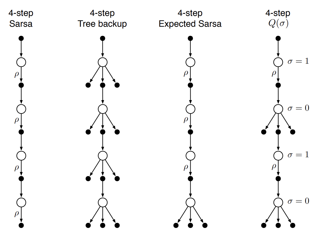Fig 5. Backup diagram of $n$-step $Q(\sigma)$.
(Image source: Sec 7.6 Sutton & Barto (2018).)

$n$-step $Q(\sigma)$ 알고리즘은 $\sigma = 1$일 떄는 sampling을, $\sigma = 0$일 때는 expectation을 나타낸다. 아래는 $n$-step $Q(\sigma)$의 $n$-step return에 대한 정의이다.

\[G_{t:h} \doteq R_{t+1} + \gamma \Big(\sigma_{t+1}\rho_{t+1} + (1 - \sigma_{t+1})\pi(A_{t+1} \vert S_{t+1})\Big)\Big(G_{t+1:h} - Q_{h-1}(S_{t+1},A_{t+1})\Big) + \gamma \bar{V}_{h-1}(S_{t+1}), \quad t < h \leq T\]

이 때 $h = t + n$이다. 재귀호출은 $G_{h:h} \doteq Q_{h-1}(S_h,A_h) \text{ if } h < T$이거나 $G_{T-1:T} \doteq R_T \text{ if } h = T$일 때 끝난다. 알고리즘은 아래와 같다.

$\text{Algorithm: Off-policy $n$-step $Q(\sigma)$ for estimating } Q \approx q_\ast \text{ or } q_\pi$

\(\begin{align*} & \textstyle \text{Input: an arbitrary behavior policy $b$ such that $b(a \vert s) > 0$, for all } s \in \mathcal{S}, a \in \mathcal{A} \\ & \textstyle \text{Initialize } Q(s,a) \text{ arbitrarily, for all } s \in \mathcal{S}, a \in \mathcal{A} \\ & \textstyle \text{Initialize $\pi$ to be greedy with respect to $Q$, or else it is a fixed given policy} \\ & \textstyle \text{Algorithm parameters: step size } \alpha \in (0, 1] \text{, a positive integer $n$} \\ & \textstyle \text{All store and access operations can take their index mod $n+1$} \\ \\ & \textstyle \text{Loop for each episode}: \\ & \textstyle \qquad \text{Initialize and store } S_0 \neq \text{terminal} \\ & \textstyle \qquad \text{Select and store an action } A_0 \sim b(\cdot \vert S_0) \\ & \textstyle \qquad T \leftarrow \infty \\ & \textstyle \qquad \text{Loop for } t = 0, 1, 2, \dotso \text{:} \\ & \textstyle \qquad\vert\qquad \text{If $t < T$:} \\ & \textstyle \qquad\vert\qquad\qquad \text{Take action } A_t \\ & \textstyle \qquad\vert\qquad\qquad \text{Observe and store the next reward as $R_{t+1}$ and the next state as $S_{t+1}$} \\ & \textstyle \qquad\vert\qquad\qquad \text{If $S_{t+1}$ is terminal:} \\ & \textstyle \qquad\vert\qquad\qquad\qquad T \leftarrow t + 1 \\ & \textstyle \qquad\vert\qquad\qquad \text{else:} \\ & \textstyle \qquad\vert\qquad\qquad\qquad \text{Choose and store an action } A_{t+1} \sim b(\cdot \vert S_{t+1}) \\ & \textstyle \qquad\vert\qquad\qquad\qquad \text{Select and store } \sigma_{t+1} \\ & \textstyle \qquad\vert\qquad\qquad\qquad \text{Store } \frac{\pi(A_{t+1} \vert S_{t+1})}{b(A_{t+1 \vert S_{t+1}})} \text{ as } \rho_{t+1} \\ & \textstyle \qquad\vert\qquad \tau \leftarrow t - n + 1 \qquad (\tau \text{ is the time whose estimate is being updated}) \\ & \textstyle \qquad\vert\qquad \text{If $\tau \geq 0$:} \\ & \textstyle \qquad\vert\qquad\qquad \text{If } t + 1 < T \text{:} \\ & \textstyle \qquad\vert\qquad\qquad\qquad G \leftarrow Q(S_{t+1}, A_{t+1}) \\ & \textstyle \qquad\vert\qquad\qquad \text{Loop for } k = \min(t + 1,T) \text{ down through $\tau + 1$:} \\ & \textstyle \qquad\vert\qquad\qquad\qquad \text{if } k = T \text{:} \\ & \textstyle \qquad\vert\qquad\qquad\qquad\qquad G \leftarrow R_T \\ & \textstyle \qquad\vert\qquad\qquad\qquad \text{else:} \\ & \textstyle \qquad\vert\qquad\qquad\qquad\qquad \bar{V} \leftarrow \sum_a \pi(a \vert S_k)Q(S_k,a) \\ & \textstyle \qquad\vert\qquad\qquad\qquad\qquad G \leftarrow R_k + \gamma\big(\sigma_k \rho_k + (1-\sigma_k)\pi(A_k \vert S_k)\big) \big(G - Q(S_k,A_k)\big) + \gamma \bar{V} \\ & \textstyle \qquad\vert\qquad\qquad Q(S_\tau, A_\tau) \leftarrow Q(S_\tau, A_\tau) + \alpha [G - Q(S_\tau, A_\tau)] \\ & \textstyle \qquad\vert\qquad\qquad \text{If $\pi$ is being learned, then ensure that $\pi(\cdot \vert S_\tau)$ is greedy wrt $Q$} \\ & \textstyle \qquad \text{until } \tau = T - 1 \\ \end{align*}\)

Summary

지금까지 $n$-step method에 대해 알아보았다. $n$-step method는 1-step TD와 MC method 사이에 해당하는 방법으로 보다 일반적인 TD method이다. 1-step TD나 MC method는 양극단에 있는 방법이기 떄문에 항상 잘 동작하지는 않는다. 특히 $n$-step TD는 1-step TD보다 복잡하고 더 많은 계산과 메모리를 요구하지만, 단 하나의 time step이 지배하는 현상에서 벗어날 수 있다는 점에서 지불할만한 가치가 있다.

$n$-step method는 $n$-step transition을 고려하는 방법이다. 모든 $n$-step method는 update를 수행하기 위해 $n$ time step만큼 기다려야 한다. $n$-step method 역시 on-policy와 off-policy method가 있다. 특히 off-policy method에는 2가지 접근법이 있다. 하나는 importance sampling을 사용해 처리하는 방법이다. 이 방법은 단순하지만 높은 분산을 가진다. 다른 하나는 tree-backup algorithm이다.

References

[1] Richard S. Sutton and Andrew G. Barto. Reinforcement Learning: An Introduction; 2nd Edition. 2018.
[2] Richard S. Sutton and Andrew G. Barto. Reinforcement Learning: An Introduction; 2nd Edition. 2020.
[3] Towards Data Science. Sagi Shaier. N-step Bootstrapping.

Footnotes

1. DevSlem. Importance Sampling. ↩

2. Reinforcement Learning: An Introduction; 2nd Edition. 2018. Sec. 7.3, p.172. ↩