Off-policy Methods with Approximation

이 포스트에서는 on-policy function approximation을 off-policy로의 확장과 이로 인해 발생하는 문제들에 대해 다룰 것이다.

Introduction

off-policy method는 behavior policy $b$에 의해 생성된 experience로부터 target policy $\pi$에 대한 value function을 학습하는 방법이다. 반대로 on-policy method는 behavior policy와 target policy가 동일한 방법이다. off-policy method에서는 일반적으로 target policy $\pi$는 greedy policy이고, behavior policy $b$는 좀 더 효과적으로 exploration을 수행할 수 있는 policy (e.g., $\epsilon$-greedy policy) 이다.

off-policy method의 문제는 크게 두가지로 나뉜다. 첫 번째는 update target (target policy 아님)과 관련된 이슈로, 이전 tabular off-policy method에서 다뤘었던 importance sampling과 관련되어 있다. 두 번째는 update distribution과 관련된 이슈로, update distribution이 on-policy distribution을 따르지 않는 다는 점이다. on-policy distribution은 semi-gradient method의 안정성에 있어 중요하다. 이 두 이슈에 대해 이번 포스트에서 다룰 것이다.

Semi-gradient Methods

이 섹션에서는 off-policy method를 간략히 semi-gradient method로 확장한다. 이 확장된 방법은 off-policy method의 첫 번째 이슈에 대해서만 다루며, 수렴이 안되어 발산할 때도 있다.

$n$-step tabular method에서 사용했던 방법을 단순히 function approximation을 사용한 weight vector $\mathbf{w}$에 대한 update로 변경한다. off-policy method는 target policy와 behavior policy의 distribution이 다르기 때문에 importance sampling 기법을 사용한다.¹ 그 중 off-policy TD(0)와 같은 알고리즘은 per-step importance sampling ratio를 사용한다.

\[\rho_t \doteq \rho_{t:t} = \dfrac{\pi(A_t \vert S_t)}{b(A_t \vert S_t)}\]

아래는 off-policy semi-gradient TD(0)로 semi-gradient on-policy TD(0)에 $\rho_t$만 추가되었다.

\[\mathbf{w}_{t+1} \doteq \mathbf{w}_t + \alpha \rho_t \delta_t \nabla \hat{v}(S_t, \mathbf{w}_t)\]

$\delta_t$는 TD error로 아래는 각각 episodic, discounted setting과 average reward를 사용하는 continuing, undiscounted setting에서의 TD error이다.

\[\begin{align*} & \delta_t \doteq R_{t+1} + \gamma \hat{v}(S_{t+1}, \mathbf{w}_t) - \hat{v}(S_t, \mathbf{w}_t) \text{, or} \tag{episodic} \\ & \delta_t \doteq R_{t+1} + \bar{R}_t + \hat{v}(S_{t+1}, \mathbf{w}_t) - \hat{v}(S_t, \mathbf{w}_t) \tag{continuing} \end{align*}\]

$\bar{R}_t$는 average reward의 추정치이다.²

action value에 대해서도 쉽게 전환할 수 있다. 아래는 off-policy semi-gradient Expected Sarsa이다.

\[\begin{align*} & \mathbf{w}_{t+1} \doteq \mathbf{w}_t + \alpha \delta_t \nabla \hat{q}(S_t, A_t, \mathbf{w_t}) \text{, with} \\ \\ & \delta_t \doteq R_{t+1} + \gamma \sum_a \pi(a \vert S_{t+1}) \hat{q}(S_{t+1}, a, \mathbf{w}_t) - \hat{q}(S_t, A_t, \mathbf{w}_t) \text{, or} \tag{episodic} \\ & \delta_t \doteq R_{t+1} - \bar{R}_t + \sum_a \pi(a \vert S_{t+1}) \hat{q}(S_{t+1}, a, \mathbf{w}_t) - \hat{q}(S_t, A_t, \mathbf{w}_t) \tag{continuing} \end{align*}\]

이 알고리즘은 importance sampling을 사용하지 않는다. tabular case에서는 action value에 대한 1-step TD method에 importance sampling을 사용하지 않는 이유가 명확했다.³ 그러나 function approximation에서는 명확하지 않다. 그 이유를 Sutton 책에서는 아래와 같이 설명한다. (솔직히 내가 이해 못했음)

With function approximation it is less clear because we might want to weight different state-action pairs differently once they all contribute to the same overall approximation.⁴

아래는 off-policy semi-gradient Sarsa의 $n$-step version이다.

\[\begin{align*} & \mathbf{w}_{t+n} \doteq \mathbf{w}_{t+n-1} + \alpha \rho_{t+1} \cdots \rho_{t+n} [G_{t:t+n} - \hat{q}(S_t, A_t, \mathbf{w}_{t+n-1})] \nabla \hat{q}(S_t,A_t,\mathbf{w}_{t+n-1}) \text{, with} \\ \\ & G_{t:t+n} \doteq R_{t+1} + \cdots + \gamma^{n-1}R_{t+n} + \gamma^n \hat{q}(S_{t+n}, A_{t+n}, \mathbf{w}_{t+n-1}) \text{, or} \tag{episodic} \\ & G_{t:t+n} \doteq R_{t+1} - \bar{R}_t + \cdots + R_{t+n} - \bar{R}_{t+n-1} + \hat{q}(S_{t+n}, A_{t+n}, \mathbf{w}_{t+n-1}) \tag{continuing} \end{align*}\]

위 첫 번째 수식에서 $\rho_k$는 $k \geq T$ ($T$는 episode의 terminal step) 일 때 $1$이다. $t + n \geq T$일 때 $G_{t:t+n} \doteq G_t$이다.

세 번째 수식에서 on-policy semi-gradient $n$-step Sarsa의 경우 average reward가 오직 $\bar{R}_{t+n-1}$이었는데 여기서는 다르다. off-policy 여서 다른 건지, 책이 오류인 건지 모르겠다.

The Deadly Triad

off-policy learning에서 발생하는 불안정성과 발산 이슈는 아래 3가지 요소를 모두 결합할 때 발생한다. 이를 the deadly triad라고 부른다.

1. Function approximation
2. Bootstrapping
3. Off-policy learning

the deadly triad 중 2가지 요소만 결합한다면 불안정성 이슈를 피할 수 있다. 따라서 위 3개 중 하나를 포기할 수 있다면 포기하는 것이 바람직하다.

먼저, function approximation은 당연히 포기할 수 없다. function approximation은 매우 큰 state space를 효과적으로 처리할 수 있는 강력한 도구이기 때문이다.

bootstrapping 없이 학습이 가능하다는 것은 이미 알려진 사실이다. 가장 대표적인 게 Monte Carlo (MC) Method이다. 그러나 bootstrapping method는 MC method에 비해 훨씬 강력하다. online으로 학습할 수 있기 때문에 훨씬 빠르고, 데이터를 효율적으로 사용하며, continuing task에 적용 가능하다. 또한 MC method는 일반적인 bootstrapping method에 비해 분산이 훨씬 크다. 따라서 bootstrapping 역시 포기하기는 어렵다.

마지막으로 off-policy learning이다. 포기할 수 있을까? off-policy method는 target policy와 behavior policy가 다르다. 이는 어디까지나 편리한 거지, 반드시 필요한 것은 아니다. 그러나 더 큰 목표를 가진 강력한 AI를 만들기 위해서는 off-policy learning은 필수적이다. agent가 하나의 behavior policy로부터 선택된 action을 바탕으로 생성된 experience를 통해 여러 개의 target policy를 병렬적으로 학습할 수 있기 때문이다.

Linear Value-function Geometry

이 섹션에서는 value function approximation을 조금 더 추상적으로 이해해 볼 것이다. 먼저, state-value function $v : \mathcal{S} \rightarrow \mathbb{R}$이 있다고 하자. 또한 function approximation을 사용하는 대부분의 경우, state 개수보다 weight vector $\mathbf{w}$의 weight 개수가 훨씬 작다.

예를 들어 3개의 state $\mathcal{S} = \{ s_1, s_2, s_3 \}$와 2개의 weight $\mathbf{w} = (w_1, w_2)^\top$가 있다고 하자. 이 경우 value function $v = [v(s_1), v(s_2), v(s_3)]^\top$를 3차원 공간 내의 점들로 표현되며, weight vector는 하위 공간인 2차원 공간으로 표현된다. 아래는 이에 대한 그림이다.

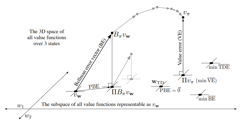Fig 1. The geometry of linear value-function approximation.
(Image source: Sec 11.4 Sutton & Barto (2020).)

위 그림에서 true value function $v_\pi$는 weight vector $\mathbf{w}$에 의해 표현되는 2차원 공간보다 더 큰 공간에 (여기서는 3차원) 표현된다.

어떤 고정된 policy $\pi$를 고려해보자. true value function $v_\pi$는 위 그림처럼 매우 복잡해서 weight vector $\mathbf{w}$로 정확히 근사하는 것은 불가능하다. 즉, $v_\pi$는 하위 공간에 존재하지 않는다. 그렇다면 표현 가능한 value function 중 어떤 것이 true value function에 가까울까?

먼저, 두 value function 사이의 거리를 측정할 필요가 있다. 두 value function $v_1$, $v_2$가 주어졌졌으며 $v = v_1 - v_2$라고 하자. 또한 특정 state를 조금 더 정확히 추정하기 위해 그 state에 얼마나 집중할 지를 나타내는 state distribution $\mu : \mathcal{S} \rightarrow [0,1]$를 (주로 on-policy distribution이 사용됨) 사용하자. 이 때 value function 사이의 distance를 아래와 같이 norm을 사용해 정의할 수 있다.

\[\big\lVert v \big\rVert_\mu^2 \doteq \sum_{s \in \mathcal{S}} \mu(s) v(s)^2\]

위 정의를 사용할 때 mean square value error $\overline{\text{VE}}(\mathbf{w}) \doteq \sum_{s \in \mathcal{S}}\mu(s)\Big[v_\pi(s) - \hat{v}(s,\mathbf{w}) \Big]^2$를 $\overline{\text{VE}}(\mathbf{w}) = \lVert v_{\mathbf{w}} - v_\pi \rVert_\mu^2$와 같은 단순한 형태로 나타낼 수 있다.⁵ 어떤 value function의 하위 공간에서의 가장 가까운 표현 가능한 value function은 projection 연산 $\Pi$을 통해 찾을 수 있다.

\[\Pi v \doteq v_\mathbf{w} \text{ where } \mathbf{w} = \underset{\mathbf{w} \in \mathbb{R}^d}{\arg\min} \ \big\lVert v - v_\mathbf{w} \big\rVert_\mu^2\]

true value function $v_\pi$에 가장 가까운 표현 가능한 value function은 $v_\pi$의 projection $\Pi v_\pi$로 Fig 1에서 확인할 수 있다.

여기서는 이정도 컨셉만 이해하고 넘어간다. 더 자세한 내용은 여기서 소개하기에는 너무 복잡해 궁금하다면 Sutton 책을 참조하기 바란다.⁶

References

[1] Richard S. Sutton and Andrew G. Barto. Reinforcement Learning: An Introduction; 2nd Edition. 2020.

Footnotes

1. DevSlem. Monte Carlo Methods in RL. Importance Sampling. ↩

2. DevSlem. On-policy Control with Approximation. Average Reward: A New Problem Setting for Continuing Tasks. Conversion to Average Reward Setting. ↩

3. DevSlem. n-step Bootstrapping. $n$-step Off-policy Learning. ↩

4. Reinforcement Learning: An Introduction; 2nd Edition. 2020. Sec. 11.1, p.259. ↩

5. DevSlem. On-policy Prediction with Approximation. The Prediction Objective ($\overline{\text{VE}}$). ↩

6. Reinforcement Learning: An Introduction; 2nd Edition. 2020. Sec. 11.4, p.266. ↩