Temporal-Difference Learning

이 포스트에서는 RL에서 반드시 알아야 하는 RL의 핵심인 Temporal-Difference learning method를 소개한다.

What is TD learning

Temporal-Difference (TD) learning method는 Monte Carlo (MC) method와 Dynamic Programming (DP)의 아이디어를 결합한 방법이다. TD method는 아래와 같은 특징을 가지고 있다.

• MC method처럼 model 없이 experience로부터 학습이 가능하다. (agent는 environment dynamics $p(s’,r \vert s,a)$를 모른다.)
• DP처럼 다른 학습된 추정치를 기반으로 추정치를 update한다. 즉, bootstrap이다.
• Generalized Policy Iteration (GPI)를 따른다.

TD method는 DP와 MC method의 치명적 단점들을 극복한 방법이다. GPI의 control에서는 약간의 차이만 있을 뿐 거의 비슷하다. 핵심은 GPI의 prediction 부분이며 여기서 큰 차이를 보인다. TD method가 어떻게 prediction을 다루는지 알아보자.

TD Prediction

TD와 MC method의 공통점은 prediction problem을 해결하기 위해 sample experience를 사용한다는 점이다. MC method의 가장 큰 단점은 value function을 추정하기 위해 return을 구해야 했기 때문에 episode의 종료를 기다려야 한다는 문제가 있었다. every-visit MC method의 value function을 추정하는 단순한 update rule은 아래와 같다.

\[\begin{align} V(S_t) &\leftarrow V(S_t) + \alpha \Big[G_t - V(S_t) \Big] \\ V(S_t) &\leftarrow (1 - \alpha)V(S_t) + \alpha G_t \end{align}\]

$G_t$는 time step $t$에 대한 return으로 MC method의 target이다. $\alpha$는 step-size parameter 혹은 weight이다. 위 update rule을 constant-$\alpha$ MC라고도 부른다.

참고로 이 포스트에서 일반적인 value function은 소문자로 (e.g. $v$) 표기하며, value function의 추정치임을 명확하게 나타낼 때는 대문자로 (e.g. $V$) 표기한다.

위의 첫 번째 update rule은 incremental한 형식으로 일반적인 형태는 아래와 같다.

\[\textit{NewEstimate} \leftarrow \textit{OldEstimate} + \textit{StepSize} \Big[\textit{Target} - \textit{OldEstimate} \Big]\]

TD method는 앞서 언급했듯이 DP의 bootstrap 속성을 가져왔다. TD method는 MC method처럼 episode의 종료를 기다릴 필요 없이 next time step까지만 기다리면 된다. next time step $t+1$에서 TD method는 즉시 target을 형성할 수 있다. 아래는 TD method의 간단한 update rule이다.

\[V(S_t) \leftarrow V(S_t) + \alpha \Big[R_{t+1} + \gamma V(S_{t+1}) - V(S_t) \Big]\]

$R_{t+1}$은 획득한 reward, $\gamma$는 discount factor이다. TD method는 reward $R_{t+1}$과 이미 존재하는 next state value 추정치 $V(S_{t+1})$을 통해 현재 state의 value function을 즉시 업데이트 한다. 특히 업데이트에 사용되는 TD method의 target을 TD target이라고 하고, TD target과 현재 state의 value 추정치와의 차이를 TD error라고 한다. 특히 TD error는 RL에서 중요한 형식으로 RL 전반에 걸쳐 다양한 형태로 나타난다.

\[\textit{TD target} \doteq R_{t+1} + \gamma V(S_{t+1})\] \[\textit{TD error } \delta_t \doteq R_{t+1} + \gamma V(S_{t+1}) - V(S_t)\]

이러한 TD method를 TD(0) 혹은 one-step TD라고 하는데 TD($\lambda$)나 $n$-step TD method의 특수 case이다. 아래는 TD(0)에 대한 알고리즘이다.

$\text{Algorithm: Tabular TD(0) for estimating } v_\pi$

\(\begin{align*} & \textstyle \text{Input: the policy } \pi \text{ to be evaluated} \\ & \textstyle \text{Algorithm parameter: step size } \alpha \in (0, 1] \\ & \textstyle \text{Initialize } V(s) \text{, for all } s \in \mathcal{S}^+ \text{, arbitrarily except that } V(\textit{terminal}) = 0 \\ \\ & \textstyle \text{Loop for each episode: } \\ & \textstyle \qquad \text{Initialize } S \\ & \textstyle \qquad \text{Loop for each step of episode:} \\ & \textstyle \qquad\qquad A \leftarrow \text{action given by } \pi \text{ for } S \\ & \textstyle \qquad\qquad \text{Take action } A \text{, observe } R, S' \\ & \textstyle \qquad\qquad V(S) \leftarrow V(S) + \alpha[R + \gamma V(S') - V(S)] \\ & \textstyle \qquad\qquad S \leftarrow S' \\ & \textstyle \qquad \text{until } S \text{ is terminal} \\ \end{align*}\)

아래는 TD(0)에 대한 backup diagram이다.

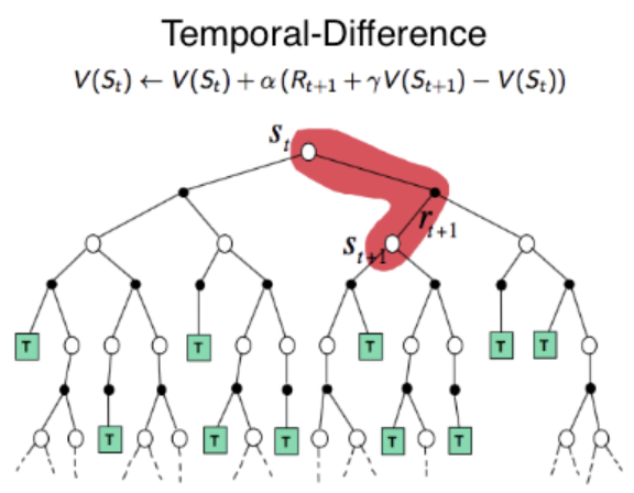Fig 1. TD(0) backup diagram.
(Image source: Robotic Sea Bass. An Intuitive Guide to Reinforcement Learning.)

backup diagram의 맨 위 state node에 대한 value 추정치는 next state로의 딱 1번의 sample transition을 통해 즉각적으로 update된다.

TD Control

우리는 앞서 TD prediction을 통해 value function을 추정하는 방법을 알아보았다. 이제 GPI에 따라 TD control을 통해 policy를 update할 것이다. MC method와 마찬가지로 sampling을 통해 학습하기 때문에 exploration과 exploitation에 대한 trade off 관계를 고려해야 하며, 이를 수행하는 방법으로 TD method 역시 on-policy와 off-policy method가 있다.

MC method에서 state value $v_\pi$를 추정할 경우 environment에 대한 지식인 state transition probability distribution을 알아야 policy improvement를 수행할 수 있었다.¹ 이는 TD method에도 동일하게 적용된다. 다행이 이러한 문제는 $v_\pi$ 대신 action value $q_\pi$를 directly하게 추정하면 해결할 수 있다. $q_\pi$를 추정하는 것의 장점은 environment에 대한 지식이 필요가 없어지는 것 뿐만 아니라 TD Prediction에서의 state value 추정과 본질적으로 같기 때문에 아래 그림과 같이 단지 state에서 state-action pair sequence로 대체하기만 하면 된다.

Fig 2. State-action pair sequence.
(Image source: Sec 6.4 Sutton & Barto (2018).)

앞으로 알아볼 TD method algorithm은 모두 action value $q_\pi$를 추정한다. 이 때 TD method는 bootstrap하기 때문에 다른 학습된 next state에서의 action value 추정치를 기반으로 현재 state-action pair의 $Q(s,a)$를 추정한다. 따라서 TD method algorithm들은 다른 학습된 action value 추정치를 고려하는 방식에 따라 구분된다. 조금 더 구체적으로 얘기하자면, TD method를 target policy와 behavior policy 관점에서 볼 때 현재 update하려는 state-action pair는 behavior policy에 의해 선택되고, 다른 학습된 action value 추정치에 대한 선택은 target policy에 의해 이루어진다. 이 target policy를 어떻게 설정하느냐에 따라 algorithm들이 구분된다.

Sarsa

Sarsa는 가장 기본적인 TD on-policy method이다. 현재 state-action pair의 action value $Q(S_t,A_t)$를 추정할 때 다른 학습된 next state-action pair에 대한 $Q(S_{t+1},A_{t+1})$을 현재 policy $\pi$에 따라 선택한다. 이에 대한 update rule은 아래와 같다.

\[Q(S_t, A_t) \leftarrow Q(S_t, A_t) + \alpha \Big[R_{t+1} + \gamma Q(S_{t+1}, A_{t+1}) - Q(S_t, A_t) \Big]\]

당연하지만 $S_{t+1}$이 terminal state일 경우 $Q(S_{t+1}, A_{t+1})$은 0이다. 위 update rule을 TD Prediction에서 보았던 TD method의 state value에 대한 update rule과 비교해볼 때 단지 state value 추정치 $V(S)$를 action value $Q(S, A)$로 대체했을 뿐임을 확인할 수 있다.

Sarsa를 target policy와 behavior policy 관점에서 살펴보자. Sarsa는 on-policy method이기 때문에 target policy와 behavior policy가 동일하다.² 따라서 next state-action pair에 대한 $Q(S_{t+1}, A_{t+1})$을 현재 behavior policy $\pi$에 따라 선택한다. 원래 behavior policy는 $b$로 나타내지만 on-policy method이기 떄문에 $\pi = b$이다. 아래는 위 update rule의 backup diagram이다.

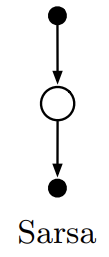Fig 3. Sarsa backup diagram.
(Image source: Sec 6.4 Sutton & Barto (2018).)

모든 on-policy method에서는 experience 생성에 사용된 behavior policy $\pi$에 대한 $q_\pi$를 추정함과 동시에, 추정된 $q_\pi$에 관해 behavior policy $\pi$를 greedy한 방향으로 update한다. Sarsa가 수렴하기 위해서는 exploration이 잘 수행되어야 하기 때문에 주로 $\epsilon$-soft policy류의 방법을 사용한다. 아래는 Sarsa algorithm이다.

$\text{Algorithm: Sarsa (on-policy TD control) for estimating } Q \approx q_\ast$

\(\begin{align*} & \textstyle \text{Algorithm parameters: step size } \alpha \in (0,1], \text{ small } \epsilon > 0 \\ & \textstyle \text{Initialize } Q(s,a) \text{, for all } s \in \mathcal{S}^+, a \in \mathcal{A}(s) \text{, arbitrarily except that } Q(\textit{terminal},\cdot) = 0 \\ \\ & \textstyle \text{Loop for each episode:} \\ & \textstyle \qquad \text{Initialize } S \\ & \textstyle \qquad \text{Choose } A \text{ from } S \text{ using policy derived from } Q \text{ (e.g., } \epsilon \text{-greedy)} \\ & \textstyle \qquad \text{Loop for each step of episode:} \\ & \textstyle \qquad\qquad \text{Take action } A \text{, observe } R, S' \\ & \textstyle \qquad\qquad \text{Choose } A' \text{ from } S' \text{ using policy derive from } Q \text{ (e.g., } \epsilon \text{-greedy)} \\ & \textstyle \qquad\qquad Q(S,A) \leftarrow Q(S,A) + \alpha [R + \gamma Q(S',A') - Q(S,A)] \\ & \textstyle \qquad\qquad S \leftarrow S'; \ A \leftarrow A'; \\ & \textstyle \qquad \text{until } S \text{ is terminal} \end{align*}\)

아래는 위 algorithm을 구현한 소스 코드이다.

Windy Gridworld³ training with Sarsa: DevSlem/rl-algorithm (Github)

Q-learning

Q-learning은 RL에서 가장 기본적이면서도 가장 중요한 알고리즘 중 하나이다. Q-learning은 off-policy TD method이며 아래와 같이 정의된다.

\[Q(S_t, A_t) \leftarrow Q(S_t, A_t) + \alpha \Big[R_{t+1} + \gamma \max_a Q(S_{t+1},a) - Q(S_t,A_t) \Big]\]

Q-learning과 Sarsa의 가장 주요한 차이는 TD error를 구성할 때 next state-action pair의 value function $Q$를 선택하는 기준이다. Sarsa는 next state $S_{t+1}$에서 현재 policy $\pi$를 따라 action value를 선택했다면, Q-learning은 현재 policy와 상관 없이 next state에서의 maximum action value $\max_a Q(S_{t+1},a)$를 선택한다. Q-learning의 backup diagram은 아래와 같으며 Sarsa의 backup diagram과 비교해보길 바란다.

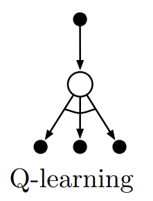Fig 4. Q-learning backup diagram.
(Image source: Sec 6.5 Sutton & Barto (2018).)

위 backup diagram에서 화살표 사이를 이어주는 선은 greedy selection을 의미한다.

Q-learning을 target policy와 behavior policy 관점에서 살펴보자. Q-learning은 off-policy method로 target policy와 behavior policy가 분리된다.² Q-learning에서 next state-action pair에 대한 value function $Q$를 고려할 때 greedy하게 고려하기 때문에 target policy는 greedy policy이다. behavior policy는 exploration을 충분히 수행할 수 있는 임의의 policy (e.g. $\epsilon$-soft policy)이다. 아래는 Q-learning algorithm이다.

$\text{Algorithm: Q-learning (off-policy TD control) for estimating } \pi \approx \pi_\ast$

\(\begin{align*} & \textstyle \text{Algorithm parameters: step size } \alpha \in (0,1] \text{, small } \epsilon > 0 \\ & \textstyle \text{Initialize } Q(s,a) \text{, for all } s \in \mathcal{S}^+, a \in \mathcal{A}(s) \text{, arbitrarily except that } Q(\textit{terminal}, \cdot) = 0 \\ \\ & \textstyle \text{Loop for each episode:} \\ & \textstyle \qquad \text{Initialize } S \\ & \textstyle \qquad \text{Loop for each step of episode:} \\ & \textstyle \qquad\qquad \text{Choose } A \text{ from } S \text{ using policy derived from } Q \text{ (e.g., } \epsilon \text{-greedy)} \\ & \textstyle \qquad\qquad \text{Take action, observe } R,S' \\ & \textstyle \qquad\qquad Q(S,A) \leftarrow Q(S,A) + \alpha [R + \gamma \max_a Q(S',a) - Q(S,A)] \\ & \textstyle \qquad\qquad S \leftarrow S' \\ & \textstyle \qquad \text{until } S \text{ is terminal} \end{align*}\)

아래는 Q-learning과 Sarsa algorithm을 구현한 뒤 비교하는 소스 코드이다.

Cliff Walking⁴ training with both Q-learning and Sarsa: DevSlem/rl-algorithm (Github)

Expected Sarsa

Expected Sarsa는 Q-learning과 유사한 알고리즘이다. Q-learning이 TD error를 구성할 때 next state-action pair들의 maximum action value를 고려했다면 Expected Sarsa는 target policy $\pi$를 따랐을 때의 next state-action pair에 대한 expected value를 고려한다. 아래 update rule을 보면 조금 더 쉽게 이해할 수 있다.

\[\begin{align} Q(S_t, A_t) &\leftarrow Q(S_t, A_t) + \alpha \Big[R_{t+1} + \gamma \mathbb{E}_\pi[Q(S_{t+1},A_{t+1}) \ \vert \ S_{t+1}] - Q(S_t,A_t) \Big] \\ &\leftarrow Q(S_t, A_t) + \alpha \Big[R_{t+1} + \gamma \sum_a \pi(a \vert S_{t+1}) Q(S_{t+1},a) - Q(S_t,A_t) \Big] \end{align}\]

Expected Sarsa는 on-policy일까 off-policy method일까? 정답은 둘다 될 수 있다이다. target policy $\pi$를 어떻게 설정하느냐에 따라 달라진다. target policy와 behavior policy가 다르면 off-policy이고 같으면 on-policy method이다. 단지 그 뿐이다. 예를 들면 behavior policy $b$가 $\epsilon$-greedy policy라고 할 때 target policy $\pi$도 $\epsilon$-greedy policy이면 $\pi = b$인 on-policy method이며 expected value는 $\epsilon$-greedy policy에 관해 계산된다. 반대로 $\pi \neq b$인 off-policy method이며 target policy가 greedy policy라면 어떨까? greedy action을 제외한 나머지 action들의 확률은 0이기 때문에 expected value는 next state-action pair에 대한 maximum action value이다. 즉, Q-learning과 동일해진다. 이처럼 Expected Sarsa는 flexible하다는 것을 알 수 있으며 모든 action들을 고려하는 expected value이기 떄문에 Sarsa에 비해 분산이 작다.

아래는 Expected Sarsa의 backup diagram이다. Sarsa와 비교했을 때 모든 action을 고려하고 있음을 확인할 수 있다.

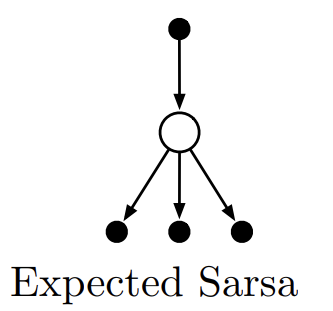Fig 5. Expected Sarsa backup diagram.
(Image source: Sec 6.6 Sutton & Barto (2018).)

Expected Sarsa는 위 Q-learning과 거의 구조가 동일하기 때문에 따로 algorithm을 올리지는 않겠다. 대신 아래에 소스코드를 첨부한다. 여기서는 target policy와 behavior policy가 동일한 on-policy Expected Sarsa를 구현했다. Expected Sarsa의 update rule은 update() 메서드에 구현되어 있다.

Expected Sarsa source code: DevSlem/rl-algorithm (Github)

Double Q-learning

기존 Q-learning의 가장 큰 문제는 biased하다는 점이다. 이로 인해 특히 stochastic한 environment에서 action value들에 대한 overestimation으로 인해 매우 나쁜 performance를 보인다. 아래 stochastic environment에 대한 예제를 먼저 살펴보자.

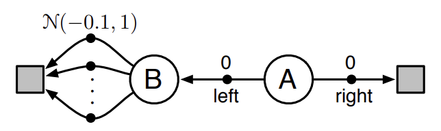Fig 6. Simple stochastic environment.
(Image source: Sec 6.7 Sutton & Barto (2018).)

agent는 항상 state A에서 시작한다. A에서 right action을 선택하면 reward 0과 함께 즉시 episode는 종료된다. left action을 선택하면 reward 0과 함께 state B로 전이된다. state B에서는 episode를 즉시 종료할 수 있는 수 많은 action들이 존재한다. 이 때 각 action들을 선택함으로써 얻게 되는 reward는 normal distribution $N(-0.1,1)$을 따른다. 즉, stochastic한 environment이다.

그렇다면 위 environment에서 왜 Q-learning은 매우 나쁜 performance를 보일까? state B에서 획득할 수 있는 reward는 $N(-0.1, 1)$을 따르기 떄문에 state A에서 left action을 선택했을 때의 expected return은 -0.1이 될 것이다. 반대로 right action의 expected return은 0이다. 그런데 Q-learning의 training 초기에 state B에서 action을 선택했을 떄 $N(-0.1, 1)$에 따라 reward를 어떤 큰 양수 (e.g. $+2$) 값으로 주로 획득했다면 어떻게 될까? training 초기이기 때문에 아직 sampling된 data가 부족해 획득된 reward의 expected value는 양수일 것이다. Q-learning은 maximum next state-action pair value를 선택한다. 이는 training 초기에 state A에서 실제 optimal action인 right가 아닌 left action을 선택하도록 유도할 것이다. 즉, training 속도는 저하될 것이다.

위 문제를 해결하도록 고안된 것이 Double Q-learning algorithm이다. 기존 Q-learning과 다르게 Double Q-learning은 action value를 2개로 나누어 추정한다. 즉, $Q_1, Q_2$를 추정하는 방법이다. 아래는 Q-learning과 Double Q-learning의 performance 비교이다. state A에서 left action을 선택하는 비율이 $y$값이며 이 값이 작을 수록 optimal하다.

Fig 7. Comparison of Q-learning and Double Q-learning.
(Image source: Sec 6.7 Sutton & Barto (2018).)

위 그림을 보면 알겠지만 Q-learning은 training 초기에 left action을 overestimation하여 left action 쪽으로 편향된 모습을 확인할 수 있다. 반대로 Double Q-learning은 training 초기부터 안정적이며 Q-learning에 비해 훨씬 빠르게 optimal에 도달한다. 이에 대한 자세한 직관적 설명은 첨부된 블로그를⁵, 수식적 증명은 논문⁶을 찾아보길 바란다.

앞서 Double Q-learning은 두 개의 action value $Q_1, Q_2$를 추정한다고 언급했다. 이 둘은 일종의 서로를 보완하는 역할을 한다. $Q_1$을 update하고 싶다고 할 때 TD error를 구성하기 위해 next state-action pair value가 필요하다. Double Q-learning 역시 Q-learning이기 때문에 target policy는 greedy policy로, next state에서 고려할 action은 $Q_1$에 대한 greedy action $A^\ast = \arg\max_aQ_1(S_{t+1},a)$이다. 기존 Q-learning에서는 TD error를 구성할 때 $A^\ast$에 대한 action value $Q_1(S_{t+1}, A^\ast)$를 고려했었다. Double Q-learning에서는 $A^\ast$에 대해 $Q_1$이 아닌 $Q_2(S_{t+1},A^\ast)$를 고려한다. 즉, $Q_1$을 update하기 위해서 $Q_2$ 추정치를 고려한다. $Q_2$를 update할 때는 반대이다. 이를 정리한 $Q_1$에 대한 update rule은 아래와 같다.

\[Q_1(S_t,A_t) \leftarrow Q_1(S_t,A_t) + \alpha \Big[R_{t+1} + \gamma Q_2\big(S_{t+1}, \underset{a}{\arg\max} \ Q_1(S_{t+1},a) \big) - Q_1(S_t,A_t)]\]

$Q_2$를 update할 때는 위 update rule에서 $Q_1$과 $Q_2$를 서로 바꿔주기만 하면 된다. $Q_1$과 $Q_2$는 당연하지만 둘이 같은 값을 가지도록 수렴할 것이다. behavior policy는 보통 $Q_1$과 $Q_2$를 모두 고려한다. 가장 간단한 방법은 behavior policy가 $Q_1 + Q_2$에 대해 action을 선택하는 것이다. $Q_1$과 $Q_2$의 update 역시 여러 가지 방법이 있겠지만 가장 간단한 방법은 각 episode의 time step $t$마다 0.5의 확률로 랜덤하게 update하는 것이다. 이에 대한 algorithm은 아래와 같다.

$\text{Algorithm: Double Q-learning, for estimating } Q_1 \approx Q_2 \approx q_\ast$

\(\begin{align*} & \textstyle \text{Algorithm parameters: step size } \alpha \in (0,1] \text{, small } \epsilon > 0 \\ & \textstyle \text{Initialize } Q_1(s,a) \text{ and } Q_2(s,a) \text{, for all } s \in \mathcal{S}^+, a \in \mathcal{A}(s) \text{, such that } Q(\textit{terminal}, \cdot) = 0 \\ \\ & \textstyle \text{Loop for each episode:} \\ & \textstyle \qquad \text{Initialize } S \\ & \textstyle \qquad \text{Loop for each step of episode:} \\ & \textstyle \qquad\qquad \text{Choose } A \text{ from } S \text{ using the policy } \epsilon \text{-greedy in } Q_1 + Q_2 \\ & \textstyle \qquad\qquad \text{Take action } A \text{, observe } R, S' \\ & \textstyle \qquad\qquad \text{With 0.5 probability:} \\ & \textstyle \qquad\qquad\qquad Q_1(S,A) \leftarrow Q_1(S,A) + \alpha \Big(R + \gamma Q_2 \big(S', \arg\max_a Q_1(S',a) \big) - Q_1(S,A) \Big) \\ & \textstyle \qquad\qquad \text{else:} \\ & \textstyle \qquad\qquad\qquad Q_2(S,A) \leftarrow Q_2(S,A) + \alpha \Big(R + \gamma Q_1 \big(S', \arg\max_a Q_2(S',a) \big) - Q_2(S,A) \Big) \\ & \textstyle \qquad\qquad S \leftarrow S' \\ & \textstyle \qquad \text{until } S \text{ is terminal} \end{align*}\)

아래는 위 update rule을 구현한 소스 코드이다. update() 메서드에 구현되어있다.

Double Q-learning source code: DevSlem/rl-algorithm (Github)

Summary

지금까지 TD method에 대해 알아보았다. TD method는 MC method와 DP의 아이디어를 결합한 방식이다. MC method 처럼 environment에 대한 지식 없이 sampling을 통해 학습하며 DP와 같이 bootstrap한 속성을 가진다. TD method 역시 GPI를 따른다. TD prediction에서 TD error는 굉장히 중요한 수식으로 RL 전반에 걸쳐 등장한다. TD method 역시 on-policy와 off-policy로 구분되며 on-policy에는 Sarsa, off-policy에는 Q-learning이 있다. 특히 Q-learning은 굉장히 중요한 algorithm이다. 그 외에도 위 두 algorithm을 개선한 Expected Sarsa, Double Q-learning을 알아보았다.

References

[1] Richard S. Sutton and Andrew G. Barto. Reinforcement Learning: An Introduction; 2nd Edition. 2018.

Footnotes

1. DevSlem. Monte Carlo Estimation of Action Values. ↩

2. DevSlem. Off-policy methods. ↩ ↩²

3. Reinforcement Learning: An Introduction; 2nd Edition. 2018. Sec. 6.4, p.152; Example 6.5: Windy Gridworld. ↩

4. Reinforcement Learning: An Introduction; 2nd Edition. 2018. Sec. 6.5, p.154; Example 6.6: Cliff Walking. ↩

5. Towards Data Science. Ziad SALLOUM. Double Q-Learning, the Easy Way. ↩

6. Hado van Hasselt. Double Q-learning. ↩